Experiment 4: Defining significance

After you have complete the previous experiments, you should have discovered that there are three different classes of organisms in the F2 generation.  Approximately

• 1 out of 4 (25%) F2 plants express, and breed true for the recessive trait.
• 1 out of 4 (25%) F2 plants express and breed true for the dominant trait.
• 2 out of 4 (50%) F2 plants express the dominant trait, but do not breed true

How do we make sense of these ratios?  Mendel's solution was to postulate that traits were determined by cellular factors; these factors were named genes by the Danish scientist Wilhelm Johannsen.

Genes can exist in different forms, called alleles.  In organisms, like peas and people, each gene is present in two copies - one supplied by the maternal parent and one supplied by the paternal parent.  The maternal and paternal alleles can be the same or different.

For example, consider flower color.  Assume that the dominant purple color is determined by the presence of the "P" allele of a specific gene .   An inbred purple parental strain has two copies of this allele - it is "PP" for the gene in question. 

The gametes that an organism produces contain one and only one copy of a particular gene.  A PP organism can only produce gametes containing the P version of the gene.

In contrast, white flower color is determined by the presence of different allele of the same gene - we will call this allele "p".  An inbred white flower parental strain is "pp" - it can produce only gametes that contain p.

If we cross true-breeding purple and white flower plants, all of the F1 off-spring with be "Pp".  These individuals can produce either of two types of gametes, ones that contain the P allele and ones that contain the p allele.

At this point Mendel made another assumption, he assumed that the chances of an F1 Pp organism producing a P gamete would be equal to its chances of producing a p gamete.   Based on this assumption, it is possible to make some very specific numerical predictions. 

Our task is to determine whether the data we find when we cross plants is consistent with these predictions or contradicts them.  This generally involves what is known as a "test for statistical significance".  

In the case of genetic data, a common statistical test is called the χ² (chi squared) test.    This test was developed by Karl Pearson (1857-1936), one of the founders of modern statistics.

In a χ² test, we begin by determining the number of "degrees of freedom" (df) in our system.   We can think of degrees of freedom as the number of measurements needed to completely define the behavior of a system.

Consider dice:  A conventional "western" die has six sides. If we know the total number of throws of the die we made, and the number of times any five of the six faces came up, we automatically know how many times the 6th side came up.   The system is therefore said to have five degrees of freedom. 

We will explore the use of the Χ² test in a set of experiments to determine whether a particular die is "fair".  First, what does fair mean?   For a standard die to be fair, the probability that it will land on any of its six faces should be equal. 

As in any experiment, we begin by forming a working hypothesis – we will assume that the die is fair, although we could also begin with the opposite hypothesis, that it is not fair.  

We choose "fair" because it makes a simpler prediction, namely that the probability of rolling a 1, 2, 3, 4, 5 or 6 will equal - we expect to see each 1/6th of the time. 

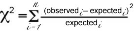
To test our hypothesis (the die is fair), we do an experiment: we roll the die some number of times and note how many times each particular face comes up.

If we roll the die 60 times, we will expect (on average) that each side will appear 10 times, BUT since a roll of the die is independent, it is extremely unlikely that we will see each side come up exactly 10 times in any 60 trials. 

How, then, do we decide whether the difference between the "expected" number of times a number appears (one in six) and the "observed" number of times it actually did appear was due to chance or to the fact that the die is unfair?  We use the Χ² formula

where "expectedi" is the expected probability that the "ith" number will appear (1/6 in our case) and "observedi" is the frequency we actually observed.

For each value, we want a positive number, so we square the difference between observed and expected. 

If expected_i = observed_i, Χ² is zero; the smaller Χ² , the more closely our observations agree with the predictions of our hypothesis.   So, how large can Χ² be before we seriously question the validity of our hypothesis? 

Because very unlikely events (like winning the lottery) do occur, we must look at our data skeptically.  (You might find the RadioLab podcast on Stochasticity/Randomness enlightening).

We are not trying to determine whether our hypothesis (about the dice) is absolute right or wrong; rather we are trying to estimate the chance that the result we observed was due to chance, even though our hypothesis was false (that is the die appears fair, even though it isn't). 

To analyze our results, we use a table of critical values, determined by the degrees of freedom in the system (df), and how stringently we seek to test our hypothesis.  

The typical standard is based on a critical value of 0.05, which means we should expect to see the results we observed strickly by chance in 1 experiment out of 20.  

If our calculated Χ² value is much smaller than this critical value, it is even less likely is due to chance, even if our hypothesis was wrong.

It is important to remember that the Χ² test helps us estimate uncertainties, it does not determine whether our hypothesis is true.

Χ²critical
values (α)

Experiment 4 directions: 

• Perform the die experiment (below) at least three separate times.
• For each trial, note the number of throws you used before you made your conclusion, the final Χ² value. 
• Did you ever observe that a die appeared to be fair after a certain number of throws and then unfair later or visa versa?  How would you explain this behavior?
• What happens as you increase the number of trials to 100 - 200?  

  ---

• Why is the hypothesis "the die is fair" easier to test than the hypothesis "the die is unfair"?
• Is it logically the case that proving that "the die is fair" is not supported by the data equivalent to proving that the "the die is unfair"?
• How might it happen that the data from one experiment appears to support a hypothesis, while subsequent experiments fail to support the hypothesis?